Precise Time-Domain Simulation of High-Order LTI Systems

When dealing with high-order systems (especially those between 12th and 20th order or higher), standard State-Space (SS) or Transfer Function (TF) models often suffer from numerical instability, leading to divergence or noise. If only the input-output response is required, the most robust approach is to discretize the system using Poles and Zeros directly and execute it using Second-Order Sections (SOS), bypassing polynomials and large matrices.

1 Principles of High-Precision Simulation

• Elimination of Polynomials (TF): Polynomial coefficients increase exponentially with the system order, making numerical precision loss (underflow/overflow) inevitable in high-order systems.
• Limits of Matrix (SS) Operations: Beyond the 12th order, matrix operations like discretization (c2d) or pole extraction (ss2zpk) begin to accumulate significant numerical errors.
• Direct Tustin Transformation (Bilinear): Mapping continuous-time poles and zeros individually to the discrete-time \(z\)-plane completely avoids the risk of conditioning issues associated with large-scale matrix computations.

2 Implementation Code for Comparative Validation

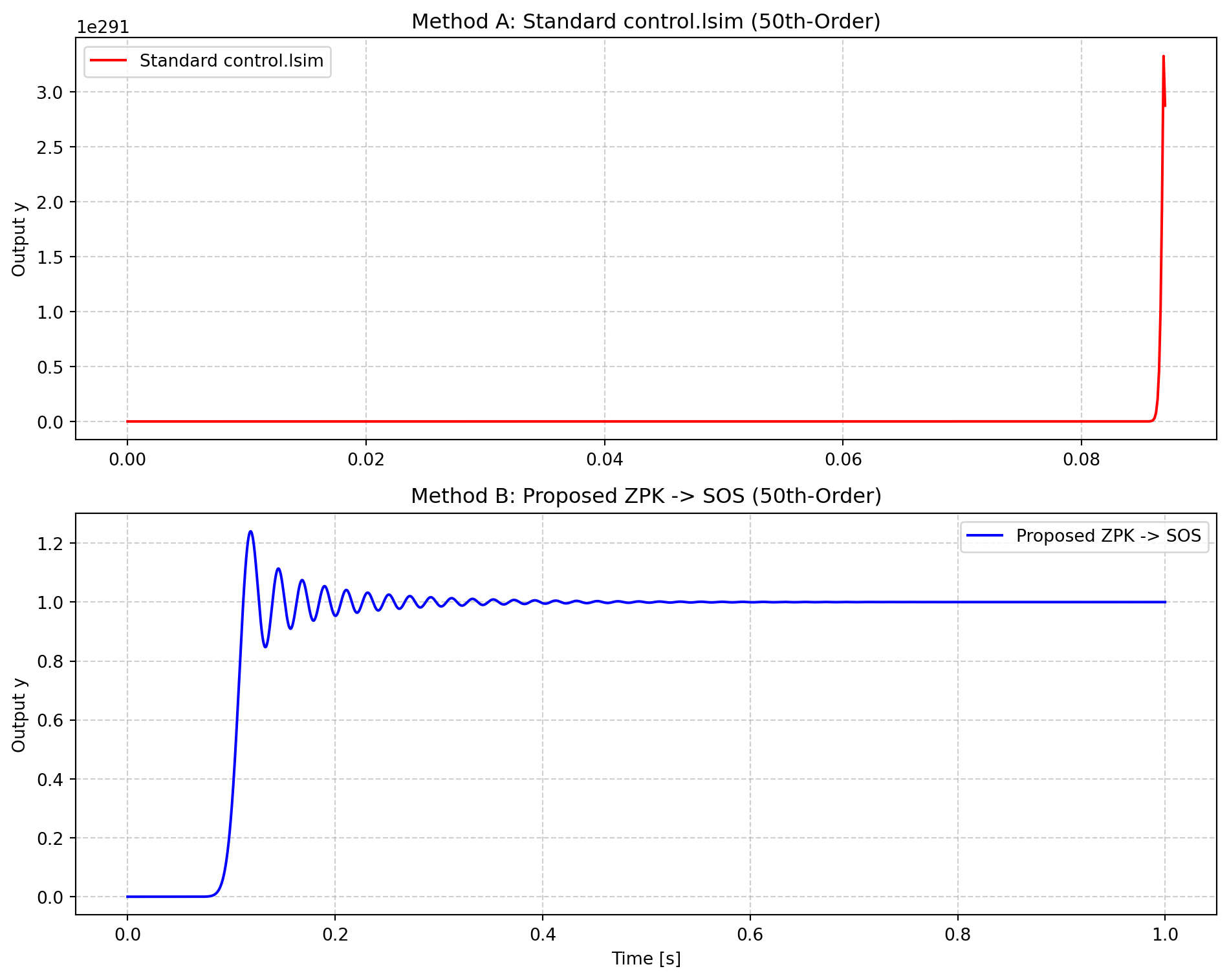
This code compares the standard control.matlab.lsim with the high-precision ZPK -> SOS (Direct Mapping Method).

import numpy as np
from scipy import signal
import control
import control.matlab as matlab
import matplotlib.pyplot as plt
import warnings
warnings.filterwarnings('ignore')

# --- 1. Configuration Parameters ---
dt = 125E-6
order = 50
fc = 50
duration = 1.0   

# --- 2. Generate Continuous-Time Model (ZPK Format) ---
# Example: Butterworth filter (representative of stable high-order systems)
z_c, p_c, k_c = signal.butter(order, 2 * np.pi * fc, analog=True, output='zpk')

# --- 3. Method A: Standard control.matlab.lsim ---
# Create continuous-time TF model
T_zpk_cont = control.zpk(z_c, p_c, k_c)
T_tf_cont = control.tf(T_zpk_cont)
T_tf_dist = control.c2d(T_tf_cont, dt, method="tustin")
t = np.arange(0, duration, dt)
u = np.ones_like(t)
# Standard solvers can be prone to small oscillations or deviations in high-order systems
y_lsim, t_lsim, xout = matlab.lsim(T_tf_dist, U=u, T=t)

# --- 4. Method B: High-Precision ZPK -> SOS (Direct Mapping Method) ---
# (1) Direct Tustin transformation (bilinear) of poles and zeros without matrix conversion
# Avoiding matrix operations prevents numerical errors by mapping points directly on the complex plane
z_d, p_d, k_d = signal.bilinear_zpk(z_c, p_c, k_c, fs=1/dt)

# (2) Convert to SOS format (Optimal pairing)
sos = signal.zpk2sos(z_d, p_d, k_d)

# (3) Execute filtering
y_sos = signal.sosfilt(sos, u)

# --- 5. Plotting Results ---
plt.figure(figsize=(10, 8))

# Upper plot: control.lsim
plt.subplot(2, 1, 1)
plt.plot(t_lsim, y_lsim, color='red', label='Standard control.lsim', lw=1.5)
plt.title(f'Method A: Standard control.lsim ({order}th-Order)', fontsize=12)
plt.ylabel('Output y')
plt.grid(True, linestyle='--', alpha=0.6)
plt.legend()

# Lower plot: ZPK -> SOS (Proposed)
plt.subplot(2, 1, 2)
plt.plot(t, y_sos, color='blue', label='Proposed ZPK -> SOS', lw=1.5)
plt.title(f'Method B: Proposed ZPK -> SOS ({order}th-Order)', fontsize=12)
plt.xlabel('Time [s]')
plt.ylabel('Output y')
plt.grid(True, linestyle='--', alpha=0.6)
plt.legend()

plt.tight_layout()
plt.show()

3 Comparison of Methods

Method	Recommended Order	Characteristics of Precision and Stability
TF (lsim)	Up to 5th	Quickly fails in high-order systems due to polynomial coefficient explosion.
SS (lsim)	Up to 10th	Requires matrix balancing. Errors become noticeable beyond the 12th order.
SS -> SOS	Up to 12th	Dependent on matrix pole extraction accuracy. Crosses the “8th-order barrier.”
ZPK -> SOS	over 50th	Handles poles and zeros directly; remains stable even for 100th+ order systems.

4 Conclusion

For input-output response analysis, the ultimate solution in Python is to “build and couple models in State-Space,” “extract Poles and Zeros (ZPK),” and then “convert directly to SOS via Bilinear transformation.”

This workflow effectively eliminates numerical divergence and artificial artifacts that typically plague lsim in high-order scenarios.